In the recent Qualifying Exam, there was a very nice (I mean, tough) problem in the Linear Optimization paper that nobody could solve. I was able to crack it two days later. Here it is:
Problem
A matrix is positive semidefinite if . Prove that if is positive semidefinte then the following system has a solution: .
Solution
where is a vector in whose entries are all 1.
Consider the following linear program
subject to
Its dual is
subject to
Observe that the dual is infeasible, because if there exists a solution such that and then this implies , contradicting the fact that A is positive semidefinite.
Since the dual is infeasible, the primal is either infeasible or unbounded. But is a solution to the primal, so it is unbounded. Thus there exists a solution such that Q.E.D.
Now that the math is done, it’s time for some story. All of us were taught that the Farkas lemma is extremely important, and thus all of us tried to use it to solve this problem, to no avail. I was particularly bugged by the condition , which we had never seen in all our exercises. The exam was on a Wednesday. Two days later, on a Friday evening, on a bus ride from school home, I was determined to solve it. Perhaps it was the motion and the rumbling sound of the bus, perhaps it was my subconscious mind having spent enough time on the problem, or perhaps it was just my shining moment, but I finally realized that means , given that . Now the next question is how do I use that in an LP? Well, I can’t use it in the constraints, so it must be in the objective function. Let’s try to . But wait, I have a constraint, so I must . And the rest is easy. That was probably one of my proudest moments in the PhD program so far.
So I’ve been thinking about the great talk by Shaowei (great ideas always make us think). Apart from the sheaf, another important thing for me is the fact that vector and function are the same thing. A function is an infinite-dimension vector, while a vector is a function that maps from {1, 2, …, n} to ℝ.
I came to understand that a function is an infinite dimension vector while studying Gaussian process (a Gaussian process is a Multivariate Normal Distribution with infinite dimension). After Shaowei’s talk, I came to understand the other way round. Now, I have the complete picture.
But a question I had is that if vector and function are the same thing, how come one is used to represent a point and the other is used to represent a collection of points? Well, we use these abstract concepts to represent specific things, but the concepts are not the things they represent. Furthermore, I reckon the symbols tell us that one point in an infinite-dimension space is the same as an infinite number of points in a one-dimensional space. I couldn’t see this connection between this two geometric objects when a coordinate system was in my head, but abstracting that out, the symbols showed the way. And with that thought, it sort of makes sense to get rid of the coordinate system….
I attended a math talk by Assistant Professor Shaowei Lin yesterday. The talk was about the history of algebraic geometry, about how Descartes came up with the coordinate system 500 years ago to symbolically represent geometric objects, about how mathematicians spent the next 500 years embracing the system only to try eliminating it over the last 100 years. And they succeeded. He talked about Bertrand Russell, Alexander Grothendiek and many great achievements of mathematics before, during and after their times. As always, his talk was very interesting and inspiring.
The term linear function has different meaning in calculus and in linear algebra, which often confuses me. Here’s the clarification, which is a note I made to myself.
In calculus, a linear function is a first degree polynomial: . Obviously, the function is called linear because its graphical representation is a line. However, in linear algebra, this function does not have the linear properties. The notion linear function, or linear transformation, is a mapping that has the following properties:
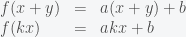
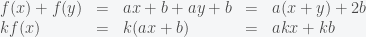
In this context, is not a linear function. To verify this, we check (1) and (2). On the left hand side,
while on the right hand side,
So both (1) and (2) are not satisfied, which shows that is not a linear function. On the other hand, we can prove easily that is a linear transformation.
The function has another name: it is an affine function, which is a linear function plus a constant.
Note that a linear transformation preserves the origin (zero is mapped to zero) while an affine transformation does not. In other words, a linear function maps a straight light through the origin to another straight line through the origin (effectively, it makes a rotation with an angle ), while an affine function rotates the line by an angle $late a$ and translate it by a distance .
In higher dimensions, what I’ve described still hold. and can be vectors in a vector space and can be a matrix.
Okay, enough with the equations. Next, I’m just gonna playing with a few functions to give you some examples.
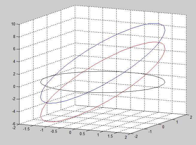
In Figure 1, the line (black) is mapped to the red line with the linear transformation and to the blue line with the affine transformation .
Figure 1
In Figure 2, the same linear and affine transformations are applied to the curve . Again, we see that the origin is preserved after the linear transformation but not the affine transformation.
Figure 2
And finally, we apply the same transformations to a circle in Figure 3.


 . Obviously, the function is called linear because its graphical representation is a line. However, in linear algebra, this function does not have the linear properties. The notion linear function, or linear transformation, is a mapping that has the following properties:
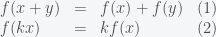
 is a linear transformation.
 ), while an affine function rotates the line by an angle $late a$ and translate it by a distance
  .
. (black) is mapped to the red line with the linear transformation
  and to the blue line with the affine transformation
  .
.
 . Again, we see that the origin is preserved after the linear transformation but not the affine transformation.


 .
.
 .
.


 . On the trigonometric circle,
  and
and  yield the same angle.